Generating categorical and continuous variables • MockData

About this vignette: This tutorial teaches the fundamentals of generating categorical and continuous variables. You’ll learn how to use create_cat_var() and create_con_var() to generate individual variables with precise control over distributions and proportions. All code examples run during vignette build to ensure accuracy.

Overview

MockData provides two core functions for generating the most common variable types:

create_cat_var() - Categorical variables (smoking status, education level, disease diagnosis)
create_con_var() - Continuous variables (age, weight, blood pressure, income)

This tutorial focuses on the basics of these two variable types. For specialized topics, see:

Missing data - Survey missing codes and NA patterns
Garbage data - Data quality testing with intentional errors
Date variables - Temporal data and survival times

Categorical variables

Categorical variables represent discrete categories with specific meanings. Examples: smoking status, education level, disease diagnosis.

Basic categorical variable

Let’s generate smoking status from the minimal-example metadata:

About example data paths

These examples use system.file() to load example metadata included with the MockData package. In your own projects, you’ll use regular file paths:
# Package examples use:
variables <- read.csv(
  system.file("extdata/minimal-example/variables.csv", package = "MockData"),
  stringsAsFactors = FALSE, check.names = FALSE
)

# Your code will use:
variables <- read.csv(
  "path/to/your/variables.csv",
  stringsAsFactors = FALSE, check.names = FALSE
)

# Load minimal-example metadata
variables <- read.csv(
  system.file("extdata/minimal-example/variables.csv", package = "MockData"),
  stringsAsFactors = FALSE,
  check.names = FALSE
)

variable_details <- read.csv(
  system.file("extdata/minimal-example/variable_details.csv", package = "MockData"),
  stringsAsFactors = FALSE,
  check.names = FALSE
)

# Generate smoking status (categorical variable)
smoking <- create_cat_var(
  var = "smoking",
  databaseStart = "minimal-example",
  variables = variables,
  variable_details = variable_details,
  n = 1000,
  seed = 123
)

# View structure
head(smoking)

str(smoking)

'data.frame':   1000 obs. of  1 variable:
 $ smoking: Factor w/ 4 levels "1","2","3","7": 1 2 1 3 3 1 2 3 2 1 ...

Categorical variable proportions

The proportion column in variable_details.csv controls the distribution of categories:

Smoking proportions from metadata:

	recStart	catLabel	proportion
5	1	Never smoker	0.50
6	2	Former smoker	0.30
7	3	Current smoker	0.17
8	7	Don’t know	0.03

Observed distribution:

# Check the distribution
table(smoking$smoking)


  1   2   3   7
505 305 160  30

prop.table(table(smoking$smoking))


    1     2     3     7
0.505 0.305 0.160 0.030

Key insight: The observed proportions closely match the metadata specifications. MockData samples categories according to the specified proportions.

Understanding categorical metadata

For smoking (cchsflow_v0002), the metadata specifies:

In variables.csv:

variableType = "Categorical"
rType = "factor" - Output as R factor with levels

In variable_details.csv:

Each category has its own row
recStart contains the category code (“1”, “2”, “3”)
proportion must sum to 1.0 across all categories

Proportion validation: Sum = 1 (must be 1.0 ± 0.01)

Continuous variables

Continuous variables represent numeric measurements on a scale. Examples: age, BMI, blood pressure, income.

Basic continuous variable (integer)

Let’s generate age from the minimal-example metadata:

# Generate age (continuous variable with integer output)
age <- create_con_var(
  var = "age",
  databaseStart = "minimal-example",
  variables = variables,
  variable_details = variable_details,
  n = 1000,
  seed = 456
)

# View structure
head(age)

str(age)

'data.frame':   1000 obs. of  1 variable:
 $ age: int  30 59 62 29 39 45 60 54 65 59 ...

Continuous variable distributions

Continuous variables use statistical distributions to generate realistic values:

# Check the distribution
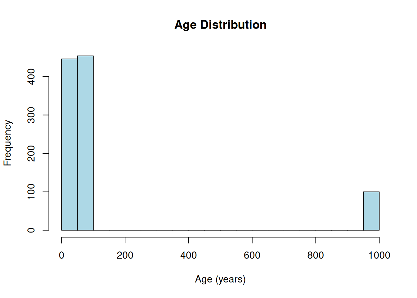
summary(age$age)

   Min. 1st Qu.  Median    Mean 3rd Qu.    Max.
  18.00   42.00   52.00  145.52   65.25  999.00

hist(age$age, breaks = 30, main = "Age Distribution", xlab = "Age (years)", col = "lightblue")

Distribution parameters from metadata:

Distribution: normal
Mean: 50
Standard deviation: 15

Interpretation: Age is drawn from a normal distribution with mean = 50 and SD = 15, truncated to the valid range specified in variable_details.csv. Notice the peak at 999—in raw data from complex sources like surveys, missing codes are often unrealistically high or low values. This is by design, but it can generate unusual patterns in the data distribution. See the Missing data tutorial for more information.

Understanding continuous metadata

For age (cchsflow_v0001), the metadata specifies:

In variables.csv:

variableType = "Continuous"
rType = "integer" - Output as whole numbers
distribution = "normal" - Use normal distribution
mean = 50, sd = 15 - Distribution parameters

In variable_details.csv:

recStart = "[18,100]" - Valid range (interval notation)
proportion = NA - Not applicable for continuous variables

The normal distribution is truncated to [18, 100], ensuring no invalid ages are generated.

Continuous variable (double precision)

Let’s generate weight, which requires decimal precision:

# Generate weight (continuous variable with double precision)
weight <- create_con_var(
  var = "weight",
  databaseStart = "minimal-example",
  variables = variables,
  variable_details = variable_details,
  n = 1000,
  seed = 789
)

# View structure
head(weight)

str(weight)

'data.frame':   1000 obs. of  1 variable:
 $ weight: num  82.9 41.1 74.7 77.7 69.6 ...

# Check the distribution
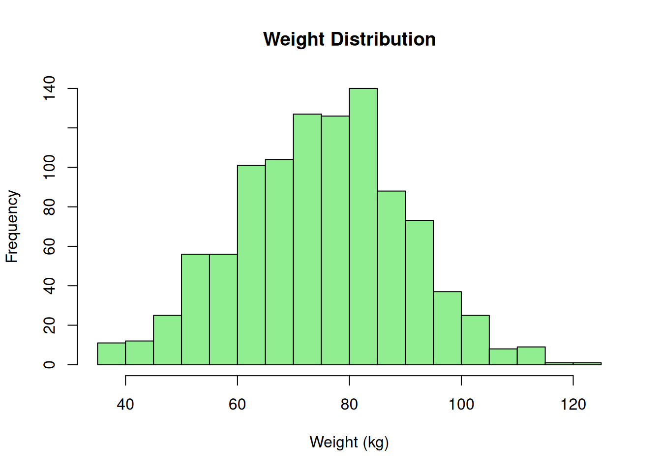
summary(weight$weight)

   Min. 1st Qu.  Median    Mean 3rd Qu.    Max.
  35.00   64.40   75.41   74.88   84.59  120.78

hist(weight$weight, breaks = 30, main = "Weight Distribution", xlab = "Weight (kg)", col = "lightgreen")

Weight parameters:

Distribution: normal
Mean: 75 kg
Standard deviation: 15 kg
Output type: double (decimal values)

Difference from age: Weight uses rType = "double" to preserve decimal precision (e.g., 72.3, 85.7), while age uses rType = "integer" for whole numbers (e.g., 45, 67).

Comparing categorical vs continuous

Aspect	Categorical	Continuous
Use case	Discrete categories	Numeric measurements
Examples	Smoking status, education	Age, weight, income
Distribution	Proportions	Statistical (normal, uniform)
variable_details	Multiple rows (one per category)	Single row (range specification)
proportion column	Required (must sum to 1.0)	NA (not applicable)
recStart	Category codes (“1”, “2”, “3”)	Interval notation (“[18,100]”)
Output types	factor, character	integer, double

When to use individual functions vs create_mock_data()

Use create_cat_var() or create_con_var() when:

Testing a single variable interactively
Exploring distribution parameters
Debugging metadata specifications
Generating variables one at a time for specific tests

Use create_mock_data() when:

Generating complete datasets with multiple variables
Need all variables generated together
Production workflows with saved metadata files

Example: Batch generation

# Generate multiple variables at once
mock_data <- create_mock_data(
  databaseStart = "minimal-example",
  variables = variables,
  variable_details = variable_details,
  n = 1000,
  seed = 100
)

# Check which variables were generated
names(mock_data)

[1] "age"            "smoking"        "height"         "weight"
[5] "interview_date"

head(mock_data[, c("smoking", "age", "weight")])

  smoking age   weight
1       1  42 88.22128
2       1  52 69.28890
3       1  49 39.45189
4       2  63 87.50134
5       1  52 57.72547
6       2  55 63.62102

Result: All enabled variables generated in a single call, maintaining consistent sample size and relationships.

Distribution types for continuous variables

MockData supports two distributions for continuous variables:

Normal distribution

Most common for naturally-varying measurements:

Parameters:

distribution = "normal"
mean - Center of distribution
sd - Spread (standard deviation)

Examples:

Age (mean = 50, sd = 15)
Weight (mean = 75, sd = 15)
Height (mean = 1.7, sd = 0.1)

Properties:

Bell-shaped curve
Symmetric around mean
~68% within 1 SD, ~95% within 2 SD
Values truncated to valid range

Uniform distribution

Equal probability across entire range:

Parameters:

distribution = "uniform"
No additional parameters needed
Uses range from variable_details.csv

Example configuration:

# variables.csv
uid,variable,distribution
v010,participant_id,uniform

# variable_details.csv
uid,variable,recStart
v010,participant_id,"[1000,9999]"

Use cases:

ID numbers
Random assignment codes
Variables without known distribution

Proportions for categorical variables

Proportions control the population distribution of categories. They must sum to 1.0 (±0.01 tolerance).

Example: Realistic smoking prevalence

catLabel	proportion
Never smoker	0.50
Former smoker	0.30
Current smoker	0.17
Don’t know	0.03

These proportions might reflect:

Published health survey statistics
Literature values for the population
Target distributions for study design

Matching published statistics

The proportion specification allows you to generate mock data that matches “Table 1” descriptive statistics from published papers.

Example scenario: A paper reports:

Never smokers: 50%
Former smokers: 30%
Current smokers: 17%
Don’t know: 3%

By setting these proportions in variable_details.csv, your mock data will match the published distribution.

Output data types (rType)

The rType column in variables.csv controls the R data type of the output:

For categorical variables

factor (recommended):

Preserves category levels
Required for statistical modeling
Example: smoking status

character:

Plain text representation
Use for IDs or non-analyzable categories
Example: participant ID, study site

For continuous variables

integer:

Whole numbers only
Use for counts, age in years
Example: age, number of children

double:

Decimal precision
Use for measurements requiring precision
Example: weight, blood pressure, lab values

Example comparison:

# Age: integer (no decimals)
head(age$age)

[1] 30 59 62 29 39 45

# Weight: double (decimal precision)
head(weight$weight)

[1] 82.86145 41.08848 74.70480 77.74710 69.57973 67.73274

Checking generated data

Always verify that generated data matches your expectations:

For categorical variables

# Check factor levels
levels(smoking$smoking)

[1] "1" "2" "3" "7"

# Check proportions
prop.table(table(smoking$smoking))


    1     2     3     7
0.505 0.305 0.160 0.030

# Verify data type
class(smoking$smoking)

[1] "factor"

For continuous variables

# Check range
range(age$age, na.rm = TRUE)

[1]  18 999

# Check distribution parameters
mean(age$age, na.rm = TRUE)

[1] 145.52

sd(age$age, na.rm = TRUE)

[1] 284.5324

# Verify data type
class(age$age)

[1] "integer"

Validation checklist:

Proportions sum to ~1.0 (categorical)
Values within expected range (continuous)
Correct data type (factor, integer, double)
Sample size matches n parameter
Distribution shape looks reasonable (histogram)

Key concepts summary

Concept	Implementation	Details
Categorical variables	`create_cat_var()`	Discrete categories with proportions
Continuous variables	`create_con_var()`	Numeric measurements with distributions
Proportions	In variable_details.csv	Must sum to 1.0 for categorical
Distributions	normal, uniform	Specified in variables.csv
Output types	rType column	factor, character, integer, double
Metadata validation	Automatic	Proportions, ranges, types checked
Batch generation	`create_mock_data()`	Multiple variables at once

What you learned

In this tutorial, you learned:

Categorical variables: Using create_cat_var() to generate variables with discrete categories
Proportions: How to specify and validate category distributions
Continuous variables: Using create_con_var() to generate numeric measurements
Distributions: Normal and uniform distributions for continuous data
Output types: Choosing appropriate rType (factor, integer, double) for each variable
Metadata structure: How variables.csv and variable_details.csv work together
Individual vs batch: When to use single-variable functions vs create_mock_data()
Validation: Checking that generated data matches metadata specifications

Next steps

Continue learning:

Date variables - Temporal data and event times
Survival data - Competing risks and censoring
Missing data - Survey missing codes (NA::a vs NA::b)
Garbage data - Data quality testing

Reference:

Configuration reference - Complete metadata schema
Getting started - Overview and first examples